
TimeScale Creator Exercises
Download Tour and Exercises here.
Let’s use TimeScale Creator to explore some interesting geologic events, and some of its other capilities.
Some of the question sets were designed for undergraduates in historical geology; but you may find them interesting.
EXERCISE #1 – Global Warming
(1) Reset display; then focus on Paleocene/Eocene boundary interval
Under FILE (top-left of menu bar); click “Replace Data with Default Datapack”. This will clear all your settings. Set up a diagram with the following: Age (use manual entry, and be sure to click that option) = (51 Ma top) to (58 base); vertical scale = 4; Geomagnetic Polarity – turn OFF; Microfossils – turn OFF. Turn ON Land Animals, open the directory and turn ON Mammals, then open it to turn ON N.Amer. zonal and selected markers, and Europe Paleogene events; and turn OFF all other Mammal columns.
Now, let’s add a title in large-font to this chart. Highlight “Chart Title” at the top of the Zonations menu. On the right-hand panel, change it to read “Paleocene-Eocene Boundary Interval”. Click the Fonts button; and for Column Header, change the Font Size to be 24 and Bold; then Close. Generate.
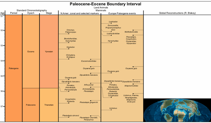
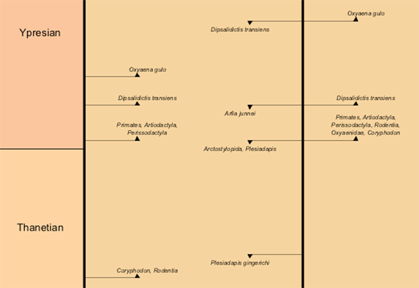
(2) Under both North America and Europe Mammals, you will see that the first appearance of Primates (early apes) occurred near the base of the Eocene epoch.
About 1 myr earlier, in North America, you see that Coryphodon (hippopotomas-looking browsers) and Rodentia (mice-squirrel-rabbit family) appeared. However notice that in the Europe column, these animals did not appear until the same time as Primates.
Therefore, one might postulate that Coryphodons and Rodentia had evolved in N. America, then migrated to Europe at the same time that Primates appeared on both continents. But, in the early Eocene, the only way for these animals to walk between North America and Europe was via land bridges to Asia that were near the Arctic-circle – notice the reconstruction. Hippopotomus-like animals could not survive such Arctic temperatures. Plus, the early Primates were tropical creatures that didn’t thrive in North America and Europe until their human descendents arrived with warm clothing. Let us investigate this question:
- What happened to cause these appearances at the beginning of the Eocene?
(3) Turn ON Sequences, Sea-level …, then under it turn OFF Sequences, Onlap … turn ON Stable Isotopes, open this sub-directory, turn ON the Cenozoic Marine Oxygen-18 Composite column. Highlight the name Cenozoic Marine Oxygen-18 Composite to bring up the menu of display options. Change the Range (initially –1 to 5) to be (-0.3 to 1.5); and click Show Scale (and make Step as 0.5). Turn off the “Show Title” for Sequences ... , and for Stable Isotopes ... by highlighting their names, as you did in Tour #3. Generate.
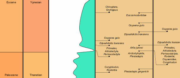
Oxygen-18 is a monitor of deep-sea temperatures, and helps indicate the temperatures in high-latitudes where these deep waters form. In an Antarctic-ice-cap-free world (which was the Eocene situation), a value of “0” is about 10-degrees C, and a value of “1” is about 6°C.
(4) This is interesting. Think about the plot, and answer the following:
- What was the general temperature trend of deep-waters from 58 million-years-ago through the earliest part of Eocene?
- What happened to bottom-water temperature at the exact time that Primates appeared in North America and Europe?
- What does this imply about the climate?
(5) Now, what caused this? Under Sequences …, then under Stable Isotopes, turn ON the Cenozoic-Mesozoic Marine Carbon-13 Composite; then, as we did with Oxygen, highlight the name Cenozoic Marine Carbon-13 Composite to bring up the menu of display options. Change the Range to be (-1 to 3); Show Scale (and make Step as 1). Generate.
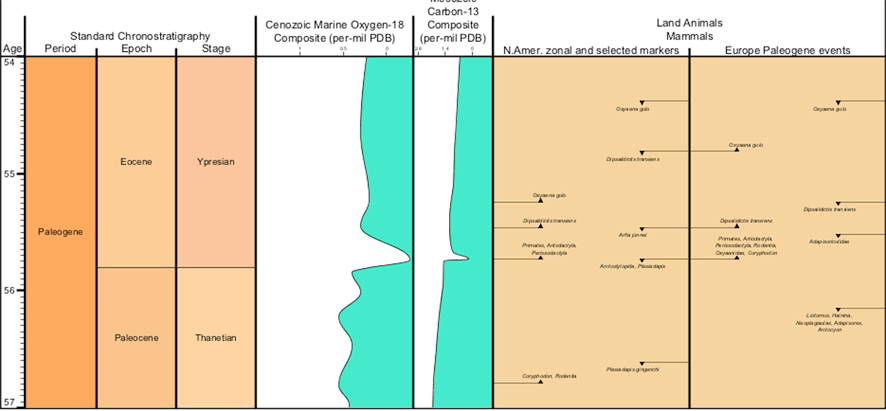
(6) Carbon-13 of organic matter is Negative, because life prefers to use Carbon-12. This is also true for coal and oil, which are derived from organic matter. Therefore, if the global-ocean becomes more “negative”, then it means that the organic carbon is being recycled back into the Earth system (especially the atmosphere). A negative shift in the Carbon-13 value by 1 is nearly equivalent to doubling the Earth’s carbon-dioxide through release of stored organic-carbon. This episode is known as the “Thermal Maximum” of the past 70 million years.
- Therefore, when you look at both the carbon and oxygen, what might have happened at the base of Eocene?
- What were the implications for mammals on the continents of North America and Europe?
- This event marked the emergence of modern mammals. Given that coincidence, then what might happen with future global warming?
(7) Possible cause. The bottom directory in Zonations menu is Impacts, Volcanism, Tectonics. Turn it ON; then open it to turn OFF Impacts and ON Large Igneous Provinces. Under Choose Time Interval menu, turn ON Add MouseOver info. Generate
The reasons for the ultra-high greenhouse and carbon-release are still debated, it appears that a massive volcanic event “North Atlantic Volcanic Province” that began the Iceland volcanic center was one of the initial triggers, followed by release of methane hydrates (very negative carbon-13 values) from ocean sediments. Click on this event to read the pop-up window, and explore more about its extent.
EXERCISE #2 – Oil in Australia
For Exercise #2 click on the icon to download the following datapack first: 
(1) Reset display; Download and add Australia Datapack
Under FILE (top-left of menu bar); click “Replace Data with Default Datapack”. This will clear all your settings.
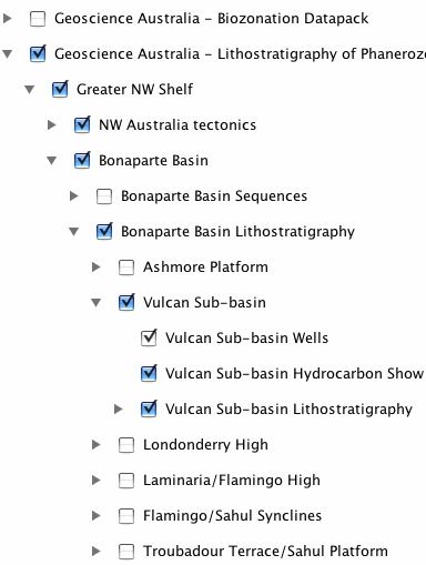
Go to the www.tscreator.org website, under Datapacks menu, download Australian biostratigraphy datapack (or follow instructions given on accessing from another class server). Unzip the file (unless it was done automatically by your operating system) to get the folder “Australia_strat_wReconstructions”. This joint product with Geoscience Australia contains lithologic columns for all major Australian basins for the past 2.5 billion years, plus all major biostratigraphy zonations and sets of tectonic reconstructions (a total of nearly 500 columns!). We will use only a small portion.
FILE (upper-left of top menu), go to Add Datapack. Using its finder, locate the folder “Australia_strat_wReconstructions”, open and load the file called “Australia_biostrat_and_basins_28Apr10.txt” (near bottom if listed alphabetically, or near top if listed chronologically). It will take a few moments to load.
Choose Time Interval of 143 to 180 Ma; with vertical scale of 1. Under Choose Zonations, turn OFF “Main Mesozoic-Paleozoic Macrofossils Groups”, “Microfossils”, and “Global Reconstructions”. Under Geoscience Australia – Lithostratigraphy of Phanerozoic Basins, turn ON “Greater NW Shelf” (and turn off the other regions). Open “Greater NW Shelf” to turn ON “NW Australia tectonics” and “Bonaparte Basin” (and turn off all other basins). Open “Bonaparte Basin” to turn ON Petrel and Vulcan subbasins (and turn off the other regions). Open “Vulcan” and turn ON “Vulcan Sub-basin Wells”. Generate.
NOTE: if you get a warning of “Don’t Panic” after Generate, then try Generate Chart again. Sometimes JAVA, especially the Windows version, doesn’t clear its memory usage very efficiently. SEE LAST PAGE for details. On some inefficient Windows operating systems, you may need to close the JAVA and restart the program.]
(2) This is a display of the geology of offshore Northwest Australia, an area that becoming a major gas-oil exporter to China and other regions.
Active “Mouse-Over”, re-Generate, and click on the Bonaparte-Basin title. In the pop-up window, click on the basin report. This opens a website at Geoscience Australia, and a summary of that basin is presented. On its right-hand menu, you can click on geologic summaries, sub-basin location maps and other items. Now, back on TimeScale Creator, use the mouse to click on one of the rock units. Again, clicking on the hot-link sends a request, in this case as a search-call their Oracle database, for information on the rock formation. You can also do this to the well-names to access a separate Oracle database of well reports. Plus, the tectonic column “light-blue” events are linked to FrOG Tech summary reports on each episode. In this fashion, the on-screen display is a “GATEWAY” into information stored on the Geoscience Australia computer databases.
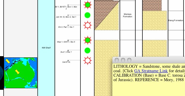
(3) On the lithology (rock) columns, you see are sands (dotted-yellow) and dark-clays (dashed brown). The red-green stars are oil-gas occurrences. The clayey Frigate Shale and Lower Vulcan Formations are organic-rich source rocks for these Jurassic oil-gas reservoirs; and the oil-gas migrated both up (into Upper Vulcan) and down (into Montara and Elang formation). Let us look at why there was this change from sands to dark shales.
(4) To save space, turn OFF Vulcan wells, NW Australia tectonics, Global Reconstructions, and Geomagnetic Polarity. Turn ON Sequences, Sea-Level …, turn ON its Sequences and T-R Cycles directory and turn ON the Phanerozoic Compilations subdirectory (only). Open that subdirectory to turn ON its Major Mesozoic-Cenozoic T-R Trends (only). This is a cartoon of global sea-level changes, in which the Blue-color indicates rising/falling ocean levels. [Turn OFF the Cenozoic-Mesozoic-Paleozoic; and to avoid excessive column titles, turn off the titles for Sequences ... and other sub-directory titles.]
Now, turn ON Stable Isotope Curves, and its Cenozoic-Mesozoic Marine Carbon-13 Composite; then, turn ON Show Scale (and make Step as 2). Turn OFF Carbon-13 and Anoxic Events. Generate.
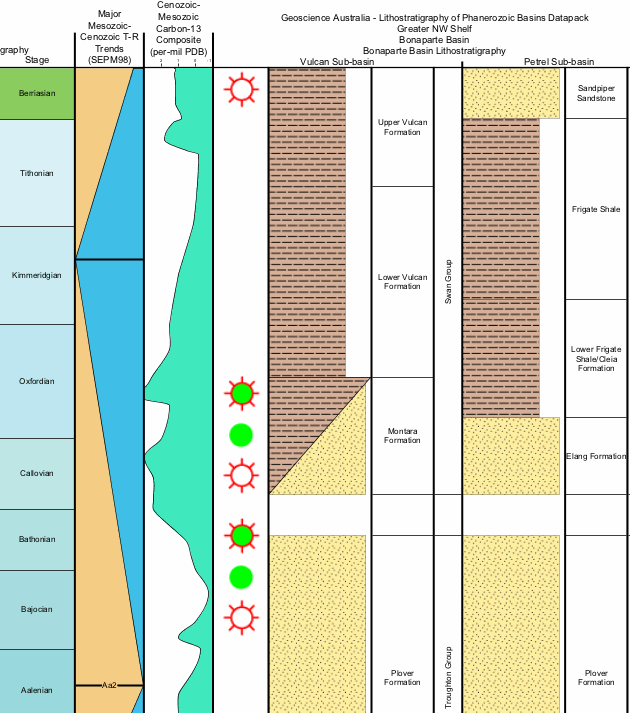
- What was sea-level doing during the onset and main part of the Lower Vulcan and Frigate Shale?
- What was it doing during the underlying main part of Plover and during the overlying Sandpiper Sandstone or Upper Vulcan?
(5) Carbon balance and sea-level. A rising sea-level causes clays and organic material to be trapped on continental shelves. Before and during the Frigate Shale, notice that the Carbon-13 curve has shifted toward the left (to more positive values). This is opposite what we saw for the base of Eocene.
- What does this imply about the global carbon system?
(6) When sea-level retreated toward the end of the Jurassic, river deltas built outward and dumped their sands onto the continental margins. These became the future oil-gas reservoirs that received the maturing hydrocarbons from the adjacent organic-rich clays. This combination of increased carbon-burial during rising global sea-level of the “Oxfordian-early Kimmeridgian” time, followed the deposition of sands during the following drop in sea-level led to the oil-gas riches of other regions, including Saudi Arabia, the North Sea and Siberia.
EXERCISE #3 – End of Pyramid civilization
For Exercise #3 click on the icon to download the datapack first: 
(1) Load our prototype for a Human Civilization time scale – From the www.tscreator.org datapack page, download the “Past 10,000 Years” datapack. Then, in TS-Creator, under FILE, click “REPLACE Data with Datapack”, and find/load the file “Past 10000 years.txt”. This completely replaces the geological scales suite with a new one of selected archeology and ice core information. This database has been compiled from both archeology sources and the independent international drilling of Antarctic and Greenland ice cores. [NOTE: it is only a preliminary sketch of what will become a major dataset in the future.]
(2) Under Settings, choose the interval spanning the Bronze Age (3.2 Ma top; 5.5 Ma bottom); and a vertical scale of 10. Under Zonations, turn OFF everything, except Age, Stage, Egypt, Egyptian Events and Middle East to India. Generate.
(3) Notice that the end of the Old Kingdom (pyramids) is simultaneous with the end of the Akkadian civilization in Mesopotamia; and there is a gap before the Middle Kingdom and Assyrian. Let us see what may have caused this.
(4) In Settings, click ON Ice-Rafting and Greenland GRIP Oxy-18. Highlight the name Greenland GRIP Oxy-18, and activate the Show Scale with a Step of 1. Generate.
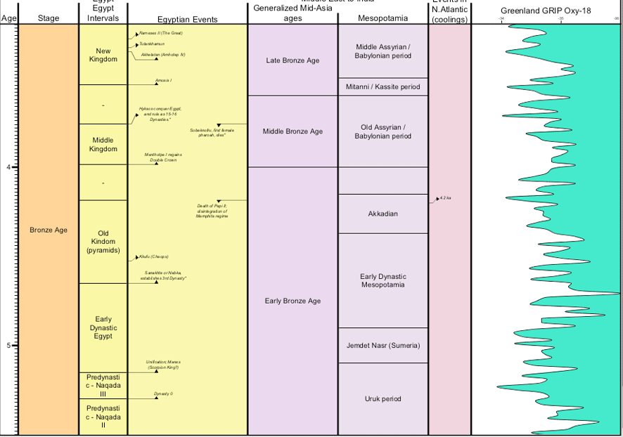
(5) A decrease in Greenland Oxygen-18 (shift to right in the diagram) is interpreted to imply that Greenland became warmer. It is thought that warm episodes that affected Greenland probably affected the entire northern hemisphere, including the region of Egypt and Mesopotamia. In contrast, a Greenland cooling is often associated with a surge in glacial icebergs, causing ice-rafting events into the North Atlantic.
- What climate event occurred near the beginning of the Old Kingdom?
- What event occurred at the collapse of the Old Kingdom and Akkadian empire in Mesopotamia?
(6) In Egypt and Mesopotamia, a warmer summer is associated with increased monsoonal rainfall and a higher Nile and Tigris-Euphrates river.
- What is a possible scenario for why the Old Kingdom and Akkadian empire simultaneously collapsed?
- Now,if you were in modern Egypt or Iraq, would you prefer global warming, or a cooler climate? It is an interesting question for climate policy.
(8) The Egyptian Events are also hot-linked with Mouse-over; and you are welcome to explore other civilizations and culture intervals.
EXERCISE #4 – Making your own datapacks
(1) Gulf of Mexico, Rupelian
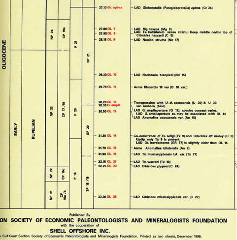
We will use the Foraminifera markers of Shell Offshore Inc. (Michael Styzen, published by Gulf Coast Section of SEPM in 1996). On the next page is a scan of just the Rupelian portion of that chart. We will make a datapack for (1) the SP “standard zones” of Shell, and (2) Shell’s “OL” foraminifer markers, which are a combination of benthic and planktonic taxa.
(2) Set-up
You will need to open EXCEL. We will be saving the file as a tab-delimited text file. Alternatively, one can use Word, and save the file as text, but this can be more tricky to easily see the tab-columns.
We will make 3 data columns: Shell SP zones, Shell Foram markers, Shell Foram details.
The format for data is quite simple.
A header that gives the column type (and optional settings for color, width, etc.)
A set of items with their ages (and optional dashed boundaries, pop-up comments, etc.)
The column sets are separated by a blank row.
(3) Block (zones)
We will enter the three SP zones with the age of their bases.
Prepare the following [NOTE: you can probably just copy-paste each set into Excel.]
The first two lines are needed to notify the program what Format is being used (1.3 allows use of separate colors for each zone, if desired)
Then, a blank row.
The “Shell SP zones” are a block-type format. Let’s use a default width of 50; and give it the bright-yellow color of Shell’s logo (RGB is 255/255/0). The seventh column (column G) can have a pop-up comment for the column title.
Each zone is entered, then its Age (as given on this SEPM chart). Notice that the lower boundary of SP21 and SP20 are dashed on the chart – but, to see how this option works, just put “dashed” after the SP20 (which has no indicated foraminifer marker). The next column (E) is for pop-up comments. For fun, let’s give zone SP 20 a light-green color (the RGB code in column F).
(4) Datums
Next, let us enter the OL “markers” as EVENTS. The column type is “event” (small letters), and the options for sets of markers are “LAD”, “FAD” and “EVENT”. We will call of these “EVENT” for now.
After a blank-row (IMPORTANT!), then enter:
The column-header above used a slightly wider width (60). Because the data-heavy event-type columns have a default of “off” to avoid accidental overcrowding of screen displays, then we’ve inserted an override of “on” in column F of the header.
Similarly, let’s compile the details of these events. There are two types used by Shell – LADs of markers, and a set of EVENTS of acme’s, co-occurrences, and transgression.
After a blank-row (IMPORTANT to have before each new header!), then enter:
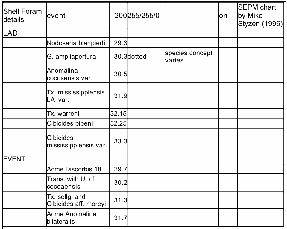
We have long taxa names, therefore a generous width of 200 units is used (column header line). The LAD of G. ampliapertura is apparently vague, therefore its marker will be dotted, and a pop-up comment is added to explain this. Note that any pop-up comments for either datums or blocks must be in column E.
Now, SAVE this Excel sheet as “TEXT (tab-delimited)” format. Use a name such as “Shell_Rupelian_Forams.txt”.
(5) Insert into TS_Creator
Let us re-set the TS-Creator to clear the previous datapack.
Under “File”, click “Replace Data with Default Datapack”.
Now, let us load the new Shell one that you’ve made – Under File, click Add datapack.
For the chart, we have a dense set of data. Therefore, under Settings (Time Interval), use Top of 29 Ma, Base of 34 Ma; and a Vertical scale of 4.
Click Generate.
Voila !! It should look like the diagram below:
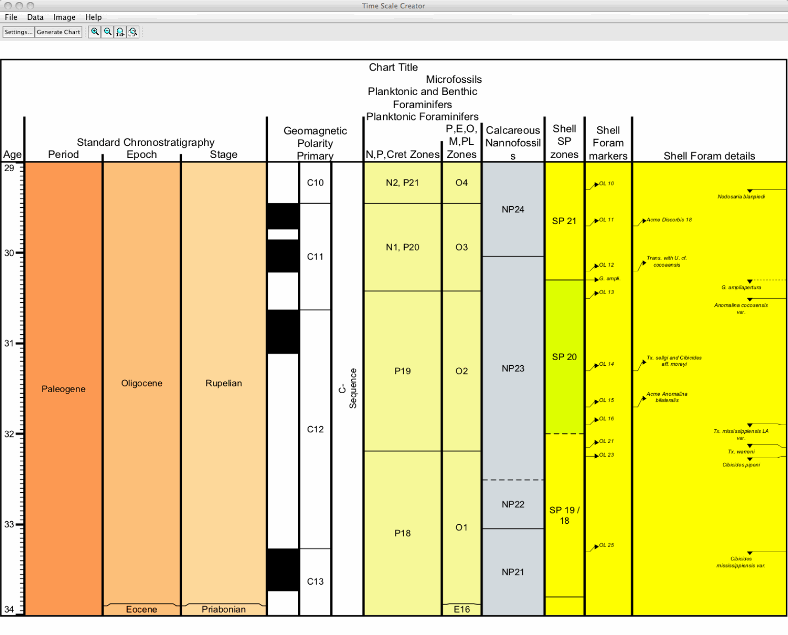
We hope this is what you get, because it should work the first time. If not, then you may see an error message indicating a problem with a certain line. This is the same line as in the Excel file, and you can open that Excel file again to see what format might be wrong. Don’t panic; just look at the instructions again, or ask us!
This completes our tour of the TimeScale Creator – a visualization system for both built-in and external databases of Earth’s history.
Additional items -- Selected display options; “out of memory”, etc.
Saving Display Parameters (Settings) – Once you’ve created a screen display that you like, then under Settings, there are bottom-buttons that enable you to SAVE … a “Settings file” that contains the necessary instructions for TimeScale Creator to recreate that display, or to LOAD … an earlier one to re-generate that same graphic for an audience or for additional revisions. If you are working on a major diagram, then we suggest using this feature to periodically save intermediate graphics, just in case the operating system has problems. This setting option is also useful to standardize diagrams (fonts, arrangements, etc.).
Details on the many other capabilities and display options are illustrated under “Features” in the Help menu (main window).
Have fun exploring the data sets and graphic options, and we hope that you will find this suite useful for reference and generating base-graphics for your research and teaching.
NOTE: The free public TimeScale Creator does not allow you to save charts after a datapack has been added. Only the PRO version allows saving charts after uploading other datasets. See our PRO page for other features, and how to get the PRO version (which comes with a large selection of datapacks).
A word of advice during exploring – there are numerous close-spaced Foram and Nanno events in the Neogene in the current database (and an abundance of Sequences in the glacial-pulsed Pleistocene), so the auto-adjust software sometimes has problems to display these details unless a vertical scale of at least 4 cm per 1 million years. A similar high-density of detail occurs with the brief North American ammonite zones in the Campanian-Turonian interval and ammonite subzones within much of the Jurassic-Cretaceous. Therefore, we have placed some of this dense-detail into “additional” columns with the lesser-used secondary events, plus shortened the genera names for the ammonites and other taxa.
A MEMORY problem that may occur -- The default Java installation on some operating systems limits the amount of memory a program can use. This Java default may cause the program to occasionally display out of memory (especially with large or information-heavy displays after several iterations). DON’T PANIC! If this happens, a message will appear on the screen -- you can still save the Settings file to regenerate the on-screen display, and usually can save the non-displayed SVG graphic file to be opened in another graphics program or Firefox-type browser. If "Out of Memory" appears, then the TimeScale Creator Pro will also explain how to increase the Java memory allocation. In many cases, hitting “GENERATE” again will solve the problem! If that doesn’t work, then before you restart TSCreator to clear Windows-memory, save your current settings (See above for SAVE/LOAD) to not loose much time.
In addition, on Window machines, the screen refresh will become slower and slower – again, the same JAVA problem in not clearing memory – so, save settings, then close and re-start JAVA and TS-Creator again.
We welcome your suggestions for major and minor improvements in the default database, visualization graphics, and overall system! Please convey your ideas, desires and critical evaluations to us at jogg@purdue.edu. Thank you, The TS-Creator team ********************************** |